Moving Average Filter: Towards Signal Noise Reduction

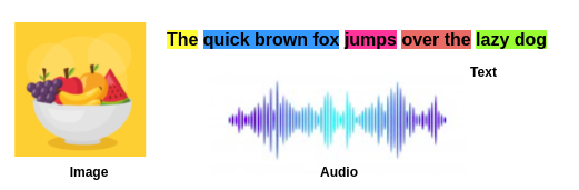
A signal is a physical quantity that varies with time, space, or other independent variables. In signal processing, a signal is a function that conveys information about a phenomenon [1]. A signal can be 1 - 1-dimensional (1D) like audio and ECG signals, 2D like images, and could be any dimensional depending upon the problem we are dealing with in general.

Signals in raw form are not always usable, we need to pass them through the filtering layer to ensure the bare minimum quality for further analysis. So first let us try to understand signal filtering and its significance, and post that will understand moving average filtering methods.

Signal Filtering

Signal filtering is a primary pre-processing step that is used in most signal-processing applications. The raw signal is not always in a usable form to perform advanced analysis i.e. various noises are present in the raw signal. We have to apply a filter in order to reduce the noise in the signal as a part of the pre-processing step.

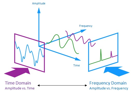
There are many pre-processing steps applied one of which is de-noising which is essential when signals are sampled from the surrounding environment. The moving average filter is one such filter that is used to reduce random noise in most of the signals in the time domain.

Now that we have understood the significance of signal filtering, let us understand the moving average filtering.

Moving Average Filter

Moving Average Filter is a Finite Impulse Response (FIR) Filter smoothing filter used for smoothing the signal from short-term overshoots or noisy fluctuations and helps in retaining the true signal representation or retaining sharp step response. It is a simple yet elegant statistical tool for de-noising signals in the time domain.

These filters are a favourite for most Digital Signal Processing (DSP) applications dealing with time-series data. It is simple, fast, and shows amazing results by suppressing noise and retaining the sharp step response. This makes it one of the optimal choices for time-domain encoded signals.

The Moving Average filter is a good smoothing filter in the time domain but a terrible filter in the frequency domain. In applications where only time-domain processing is present Moving average filters shine, but in applications where information is encoded in both time and frequency or the frequency domain solely it can be a terrible option to choose.

Types of Moving Average Filter

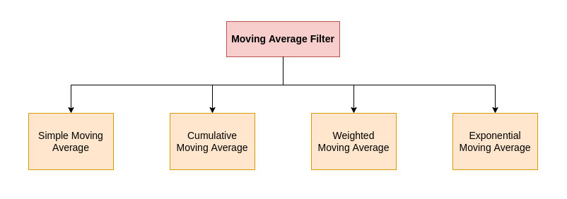
There are various types of moving average filters but on a broader level simple, cumulative moving average, weighted moving average, and exponentially weighted average filters form the basic block for most of the other variants. There are many moving average filter variants, more or less the fundamental structure boils down to four core types illustrated below figure.

This article will cover most of them on a broader level and will show use cases of it, we will also understand their variants which we had used in our research use case, and boosted performance metrics.

Now let us, deep-dive, into each of these types along with code snippets and some basic mathematical formulation.

Don’t get intimidated by coding and mathematics I have tried to keep it short and simple.

Simple Moving Average (SMA)

This is one of the simplest forms of moving average filter that is easy to understand and apply to the desired application. The main advantage of the simple moving average is that we don't need exorbitant mathematics to understand it i.e it can be interpreted by its formula itself.

The con of SMA is that it gives equal weightage to all samples due to which it does not suppress the noisy signal effectively.

Let's take an example.

Let's say we have an array of numbers \(a_{1}, a_{2}, ..., a_{n}\)

If we take periodicity (window length) as k, then the average of 'k' elements would be

For easy understanding, let's assume k = 4

\(SMA_{1} = \frac{a_{1}+a_{2}+a_{3}+a_{4 }}{4}\)

\(SMA_{2} = \frac{a_{2}+a_{3}+a_{4}+a_{5 }}{4}\)

\(\vdots\)
\(SMA_{N-k+1} = \frac{a_{n}+a_{n-1}+a_{n-2}+a_{n-3 }}{4}\)

So simple moving average filter equation result would be

SMA Array = \([SMA_{1}, SMA_{2}, \cdots, SMA_{N-k+1}]\) which contains 'N-K+1' elements.

Let us implement this simple moving average filter using Python. We will be using the convolution concept for convolving the input signal with all ones with the given window size.

import numpy as np


def simple_moving_average(signal, window=5):
    return np.convolve(signal, np.ones(window)/window, mode='same')

We will choose a simple sine wave and superimpose random noise and demonstrate how effective is a simple moving average filter for reducing noise and restoring to the original signal waveform.

Fs = 8000 # sampling frequency = 8kHz
f = 5 # signal frequency = 5 Hz
sample = 8000 # no. of samples
time = np.arange(sample)
original_signal = np.sin(2 * np.pi * f * time / Fs)   # signal generation
noise = np.random.normal(0, 0.1, original_signal.shape)
new_signal = original_signal + noise

Following is the plot showing the effectiveness of the simple moving average filter for random noise reduction:-

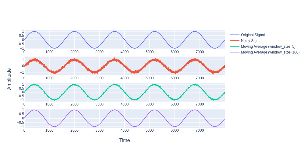
One characteristic of the SMA is that if the data has a periodic fluctuation, then applying an SMA of that period will eliminate that variation (the average always contains one complete cycle). But a perfectly regular cycle is rarely encountered.

Cumulative Moving Average (CMA)

CMA is a bit deviated from other types in moving average family and the usability of this filter in noise reduction is nil. One benefit of CMA is that it also accounts for past data considerably by also accounting for the recent data point, unlike SMA which will be just an average of past data points within a defined sliding window size and equal weights.

The simple moving average has a sliding window of constant size k, contrary to the Cumulative Moving Average in which the window size becomes larger as time passes during computation.

\[CMA_{n} = \frac{x_{1}+x_{2}+\cdots+x_{n}}{n}\]

To reduce computational overhead we use a generalised form:-

\[CMA_{n+1} = \frac{x_{n+1}+n.CMA_{n}}{n+1}\]

This is called cumulative since the ‘n+1’ terms will also account for the cumulative of ‘n’ previous data points while averaging the points.

import numpy as np


def cumulative_moving_average(signal):
    cma = []
    cma.append(signal[0]) # data point at t=0

    for i, x in enumerate(signal[1: ], start=1):
        cma.append(((x+(i+1)*cma[i-1])/ (i+1)))
 
    return cma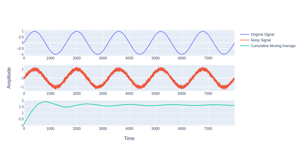

It is very evident that CMA is not at all useful for reducing noise since the retrieved signal is nowhere as pristine in shape as the original signal. This filter is worst to be used for reducing noise pursuit.

CMA is quite alien in terms of output as compared to its other family members.

But what we can learn from its formula and concept is we can give certain weights not necessarily equal i.e. playing with weights and adjustments that was a setback in the case of SMA. This is where our next topic will come into play Weighted Moving Average.

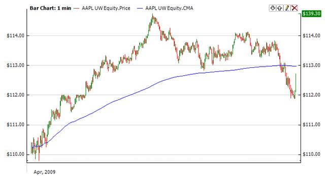
One of the interesting applications is in the stock market where data stream arrives in an orderly manner, an investor may want the average price of all trades for a particular financial instrument up until the current time. As each new transaction occurs, the average price at the time of the transaction can be calculated for all transactions up to that point using the cumulative average [3].

Weighted Moving Average

Weighted Average works similarly to that of a simple moving average filter, where we are considering the relative proportion of each data point within a window length. SMA is unweighted means while WMA contains weight for relative proportion adjustments which makes it even more captivating for application.

Let's take an example to get a better understanding of this. Let's say we have an array of numbers \(x_{1}, x_{2}, \cdots, x_{n}\). Let's keep the periodicity or window length the same as in the previous example i.e k =4

The general Weighted Average formula is

\[W = \frac{\sum_{i=1}^{n} w_i\cdot x_i}{\sum_{i=1}^{n} w_i}\]

The purpose of giving weights is to give more importance to a few data points over the other data points. And this weight depends on the application. One of the applications is in image processing to specify the filters we use. Those filter coefficients are nothing but the weights and the local patch of pixel values to which the filters are being applied serves as the data points and the combination serves as the weighted average. There are many filters for example blurring filters (nothing but equally weighted filters).

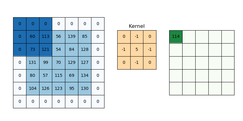
The characteristics of weights will decide what effects we want given the input samples. It is quite interesting to understand this part as it is some transformation it does with input samples to get a different perspective of input samples in a much better format and the result is better interpretability.

These WMA techniques are also being used extensively in stock markets but more than this its better variant is used like EWA or EWMA.

Exponentially Weighted Average (EWA) or Exponential Weighted Moving Average (EWMA)

An exponentially weighted average gives more weightage to recent data points and less to previous data points overall. This ensures the trend is maintained by still accounting for a decent portion of the reactive nature of recent data points. In comparison with SMA, this filter suppresses noisy components very well i.e. effective and optimal in de-noising signals in the time domain. It is 1st order infinite impulse response(IIR) filter.

The general formula is

\[\begin{equation*}EMA_t = \left\{ \begin{array}{ll} x_0 & \quad t = 0 \\ \beta \cdot x_t + (1-\beta) \cdot EMA_{t-1} & \quad t \geq 1 \end{array} \right. \end{equation*}\]

For different applications, the beta coefficient definition changes but overall the meaning remains the same giving more importance to recent data points and less to previously averaged data points.

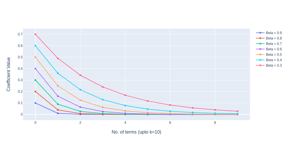
The EWMA is a recursive function, recursive property leads to exponentially decaying weights.

\[\begin{equation*}EMA_t = \beta \cdot x_t + (1-\beta)\cdot EMA_{t-1} \end{equation*}\]

\[\begin{equation*}EMA_t = \beta \cdot x_t + (1-\beta)\cdot (\beta \cdot x_{t-1} + (1-\beta)\cdot EMA_{t-2}) \end{equation*}\]

\[\begin{equation*}EMA_t = \beta \cdot x_t + \beta \cdot x_{t-1}  - \beta^2 \cdot x_{t-1}+(1-\beta)^2\cdot EMA_{t-2} \end{equation*}\]

\((1-\beta)^k\) will keep on exponentially decaying as shown in the figure below.

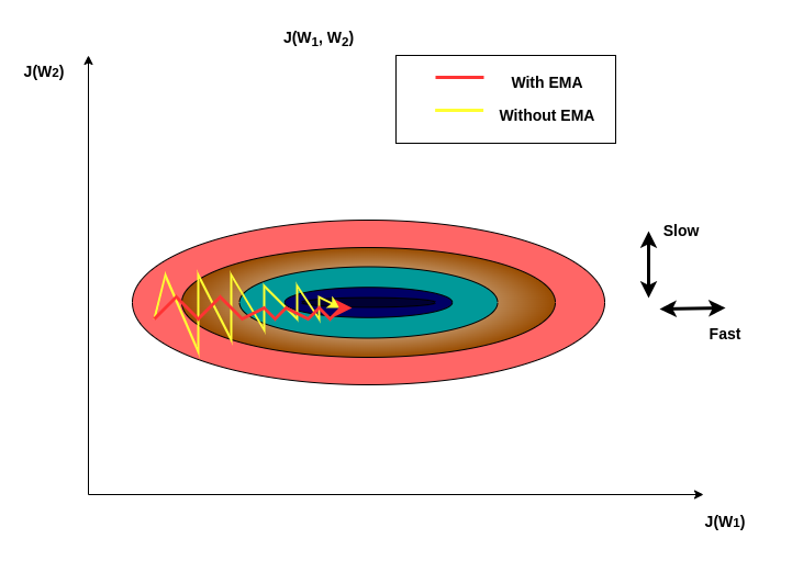
The significance of this EWMA or EMA in deep learning is known by very few people. The variants of this specific filter have been used in Deep Learning optimisers for faster convergence to global minima because the loss landscape is highly stochastic especially when the data dimension is enormous, for the optimiser to converge faster with the optimal converging path by giving relative importance to the recent path to trace out a future path while making sure the new averaged data points doesn't deviate too much from past data points. So it tries to maintain momentum while still avoiding any overshoots refer to the below figure.

This type of moving average filter has excellent usage in many other fields like in the stock market where it is considered to be one of the most simple and reliable indicators to do analysis and make decisions. It is also used in many machine learning research. There are a good number of moving average filter examples.

In one of our research use cases for efficient peak detection in ECG signals, we used a moving average filter to suppress noise and it incredibly boosts the peak detection performance. But we need to be sure about where we are using this kind of filter, especially where frequency domain operations are involved it's better to avoid this filtering.

Comparative Study

Now that we have a good understanding of the Moving Average filter we will dive into more analytical aspects of those filters. We will compare moving average filters w.r.t  Savgol filter a time-domain smoothing filter and will compare its performance.

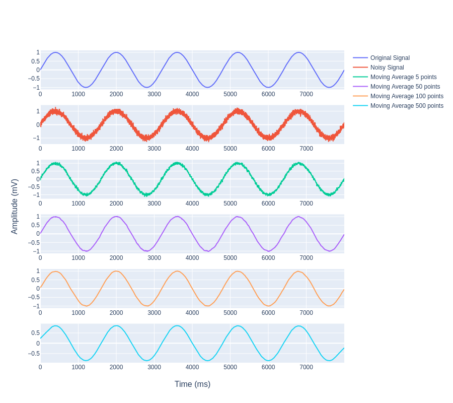
As we know moving average filters smoothen out the signal. The smoothing effect is inversely proportional to the window length i.e. the larger the window length (up to a certain limit) the clearer the signal or more the de-noising. The following figure shows this relationship clearly. We have used Gaussian white noise with sigma = 0.1. From the plot, it is apparently clear that taking 500 points averaging works really well, the signal is quite smoother and resembles that of the original signal.

Now let's understand how effective the moving average filter is when the noise factor is more.

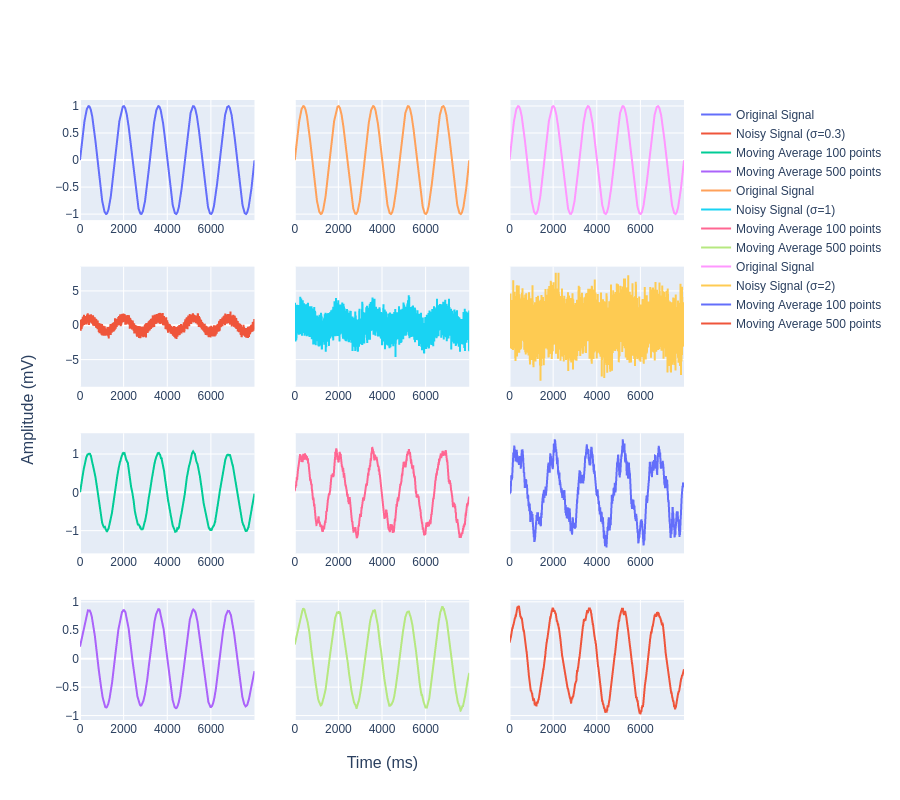
We can see in Fig 11. that there is a large amount of white noise which was added to the signal still after applying the moving average filter we are able to retrieve the original signal envelope i.e. we are able to filter out the noise effectively.

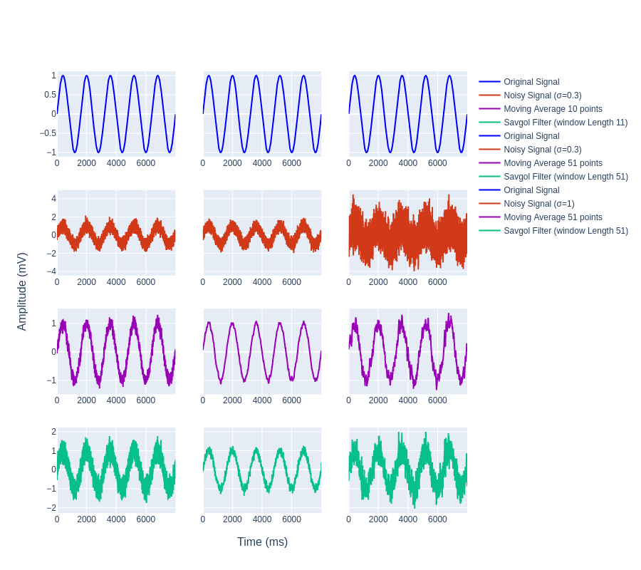
Now let us compare the smoothing effect of the simple moving average filter with that of the Savitzky–Golay filter is also known as the Savgol filter. Savgol filter increases the precision of data without much distortion in signal tendency [4]. It is one of the most widely used smoothing signal methods.

Clearly, we can see how the SMA filter retrieves the original signal envelope even with a much stronger white noise addition too. This is really suitable for Digital Communication.

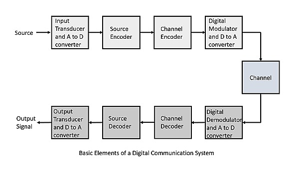
We can characterise the noise in the channel as Gaussian white noise (Gaussian white noise is a type of random signal where the amplitude of the noise at each point in time follows a Gaussian (normal) distribution, and it has a flat power spectral density, meaning it has equal power across all frequencies). We can retrieve signal shape by smoothing out the signal or removing Gaussian white noise. In digital communication, it is important to consider the Shannon Channel Capacity Limit [5] since moving the average filter is less effective for a low Signal-to-Noise ratio (Signal-to-noise ratio (SNR) is a measure of the strength of a signal relative to the background noise level). But moving average filter is a basic filtering technique applied in most communication systems to reduce the impact of white noise (white noise is a random signal with a flat power spectral density, meaning it has equal power across all frequencies within a specified range).

Moving Average filters have many potential applications. Since the Moving average filter is an excellent time-domain filter but has an inferior response in the frequency domain it is important to consider the application before applying it. So, in applications where one is dealing with spectral features (or Frequency domain operations), it is best to avoid applying moving average filters in the spatial or time domain. Also, it is best to avoid this filtering technique when analysing sharp transient signals and non-stationary signals since that would lead to a loss of details.

I hope you find this blog educative and interesting in theoretical as well as practical aspects.

Cheers to filtering noise ahead!

Want more insights and expert tips? Don't just read about Moving Average Filters! Work with brilliant engineers at Codemonk and experience it's effective use case firsthand!

References

1. Signal Introduction
2. Convolution
3. Cumulative Moving Average
4. Savitzky–Golay_filter
5. Shannon Limit