A Gentle Introduction to Multi-Objective Optimisation

Most of the tasks in machine learning have a single objective function, for example, image classification, image captioning, movie rating, etc. But there are several complex problems like Drug discovery, Hyperparameter Tuning, where a single objective function does not suffice to get the optimal solution in the solution space. This is where multi-objective optimisation comes into the picture.

Before we get into the brief overview of Multi-Objective optimisation and its incredible applications, let us dive a little bit into understanding optimisation first, followed by single objective optimisation and then finally dive into multi-objective optimisation.

Optimisation and Single-Objective Optimisation

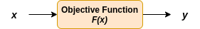
All deep learning algorithms use an optimisation algorithm that helps the network maximise or minimise an objective function depending on the use case. In general, optimisation refers to the task of either minimising or maximising some function F(x) by altering x, where 'x' is input [1].

For example, we want to build a dog 🐶 vs cat 😺 image classification model. We have prepared the dataset. We want the model to accurately classify the image, which means we want maximisation of model prediction accuracy; in another way, we can also redefine my objective by saying we want minimisation of the loss. Whether we want to maximise the accuracy or minimise the loss, the objective of the model is achieved. So the objective is only one. This is known as Single-Objective Optimisation.

Multi-Objective Optimisation

In multi-objective optimisation problems, we try to optimise many objective functions simultaneously while trying to find a balance between all competitive objective functions without many trade-offs. However, it is tough to narrow the solution search to one optimal solution since there are many feasible solutions in the solution space, and some problems have intractable solution space.

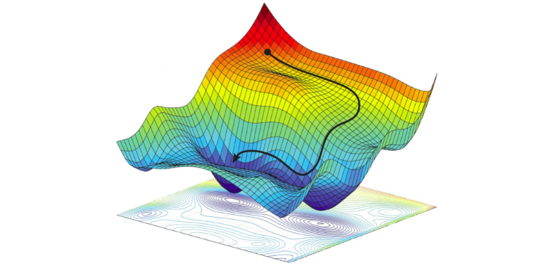
Thus, whenever we deal with Multi-Objective Optimisation, we need to have some tools to analyse the solution space and make the optimal choice as per the problem. Sometimes for specific use cases, to find an optimal solution, domain knowledge plays a pivotal role in selecting the solution considering the trade-offs. For example, in Drug Discovery, one must consider several variables like stability, effectiveness, toxicity, etc. So, often linear 1D optimisation fails to cover the optimal solution considering many objectives.

Problem with Linear 1D Optimisation

Now there might be a question, "What is the problem with single optimisation or 1D optimisation?" well, the shortcomings of 1D optimisation on multi-objective tasks are that we often land upon different solutions when trying to optimise one objective function over another. So, for example, let's say we have two objective functions, so if we apply the 1D optimisation method, we have to apply it to one objective function at a time i.e 1D optimisation on the objective-1 keeping the objective-2 constant or hidden, once the objective-1 is optimised we then apply optimisation on objective-2. So we get an optimal value which might not be the same as following the same process but this time first optimising objective-2 and then objective-1. So rather than a narrow view, we want a Bird's Eye View of a solution space to find an optimal solution.

Let's take the example of buying a car to understand this problem in a more crystal clear way. Let's say my objective is to buy a good mileage, low-cost car. The X-axis represents 'Mileage' as we move towards right from the origin, the better the mileage. The Y-axis represents the 'Cost' of the car; as we move upward, cost decreases. So we name X-axis & Y-axis 'Good Mileage' & 'Low-Cost' to better understand the concept.

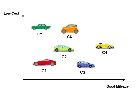
Essentially, we have to minimise cost and maximise mileage for our use case. Applying linear 1D optimisation in multi-objective tasks is like treating one dimension as hidden from an understanding point of view.

We have the following scenarios -

1. Scenario 1: Applying 1D optimisation on objective-1 i.e. Good Mileage first, followed by application of 1D optimisation on objective-2, i.e. Low-Cost.
2. Scenario 2: Applying 1D optimisation on objective-2, i.e. Low-Cost first, followed by applying 1D optimisation on objective-1, i.e. Good Mileage.

Let's make one more assumption for understanding the concept in a much better way, the car showroom is dark, and I am holding a torch to find my desired car, i.e. low cost & good mileage (I know nobody wants to buy their desired car this way 😂).

Scenario 1: Good Mileage followed by Low Cost

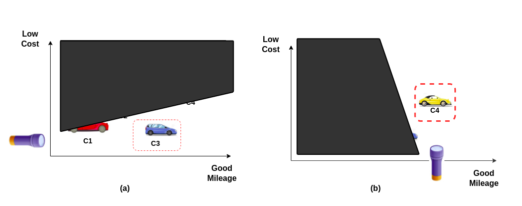
1. Referring to the above (Fig. 3 (a)), we want a car with good mileage, so we will turn 'ON' the torch and move towards the last car we can see i.e. car 'C3'.
2. After we know we have arrived at the best Mileage Car (given the torch visibility) in the showroom, the second objective is to find a low-cost car, so we will turn my torch towards that side (refer to Fig 3. (b)).
3. The only car we can find is the car 'C4'.

Scenario 2: Low Cost followed by Good Mileage

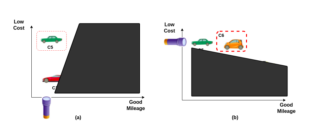
1. Referring to the above (Fig. 4 (a)), we want a car which is low cost so we will turn 'ON' the torch and move towards the low-cost car we could see i.e car 'C5'.
2. We know now that we have arrived at the best low-cost car possible (given the torch visibility) in the showroom. The second objective is to find a good mileage car, so I will turn my torch towards that side (refer to Fig 4 (b)).
3. The only car we can find is the car 'C6'.

Below is the summarised table of the two scenarios discussed so far:-

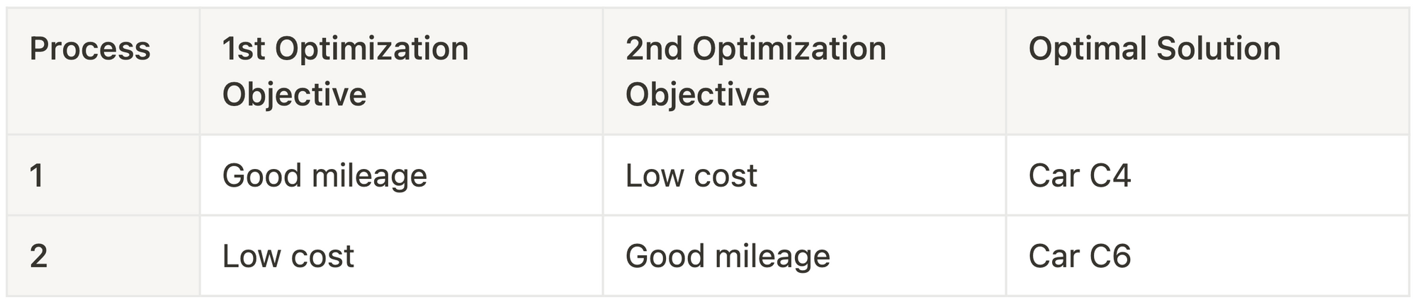
It's weird, right 🤔? So in scenario 1, we got car C4, and in scenario 2, we got car C6.

So if we choose to go with the 1D optimisation method, we might get a different solution using a different strategy.

We can conclude from Table-1 that we get different optimal solutions for different optimisation strategies. This is the major drawback of 1D optimisation for multi-objective tasks.

This is the reason why in this type of problem, Bird's Eye View is more beneficial.

Now that we have understood the setbacks of linear 1D optimisation on multi-objective tasks, let's understand different approaches to solve the same.

Types of Multi-Objective Optimisation Approaches

On a broader level, multi-objective optimisation can be achieved using two approaches.

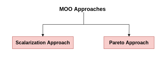
Scalarization Approach: The scalarization approach creates multi-objective functions made into a single solution using weights before optimisation.

The mathematical formulation of the Scalarization approach is as follows -

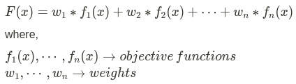
The weight of the objective function will determine the optimal solution and show us the performance priority (Refer to [4] for more details).

Pareto Approach: There is a dominated solution and a non-dominated solution obtained by a continuously updated algorithm in the Pareto approach. Let's understand a bit more about this approach.

Pareto Approach

Before understanding the Pareto concept, let us understand the dominance test.

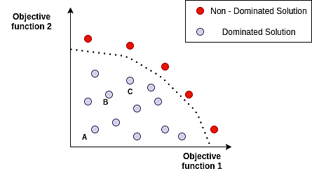
Dominated solutions are solutions that are not the optimal ones, i.e. there exist other points which supersede that point. For example, in Fig 6, point 'A' is dominated by point 'B', and point 'C' dominates both 'A' and 'B'. The solutions which cannot be dominated by any point in the feasible solution space are called 'Non-Dominated Solutions', also known as Pareto Efficient.

The Non-Dominated solution set is called Pareto Optimal Solutions/Set. Pareto Front is the boundary defined by the set of all points in objective space or criterion space mapped from the Pareto Optimal Set in decision space, refer to Fig 7. Once we find the Pareto Solution, we can apply other algorithms on top of it rather than computing the intractable solution space we curtailed to a finite set. Pareto optimal solutions are sometimes referred to as "Non-Inferior" solutions.

Once we have defined the variables, the dominance concept will be used to segregate non-dominated from dominated ones during the optimisation process. This optimisation process will continue until an optimal value is reached where we cannot improve one objective function without worsening the other. This state is referred to as Pareto Optimality. We call the solutions Pareto Optimal solutions (for more details, refer to [4]).

Broadly the different types of algorithms that are improvements to basic MOO are as follows -

1. Classic MOO methods
   a. Weighted Sum method (Refer to [5] for more details on slide 10)
   b. ε-constraints method (Refer to [5] for more details on slide 15)
   c. Weighted metric method (Refer to [5] for more details on slide 18)
   d. Global Criterion Approach (Refer to [6])
   e. Goal Programming (GP) (Refer to [6])
2. MOO using Genetic Algorithms (MOGAs) (Refer to [5] for more details on slide 22)
3. MO Evolutionary Algorithms (MOEAs) (Refer to [5] for more details on slide 25)
   a. Non-Elitist MOEAs
   b. Elitist MOEAs

Applications

There are many amazing applications of Multi-Objective Optimisation like Drug Discovery/ Design [8], Ranking problems [9], Routing Optimisations [10], Hyper-parameter Tuning, selection of relays in the ad-hoc networks [4], and many more.

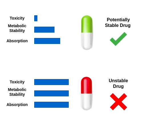
Specifically, in a drug discovery case, to discover a new drug for a particular disease there are various properties such as thermostability, absorptivity, permeability, binding, potency, toxicity, penetration, etc. These properties are essential as we want the drug to be stable, should not be toxic, and should be highly effective. This is just an example of how each of these properties is an objective function in itself and needs to be treated in a multi-objective fashion to get a desirable chemical drug.

It is captivating to see the potential application of multi-objective optimisation algorithms.

I hope you understood some of the fundamental underpinnings required to understand Multi-Objective Optimisation problems. Cheers to further exploration in MOO 🥂.

Want more insights and expert tips? Don't just read about Multi-Objective Optimisation! Work with brilliant engineers at Codemonk and experience it's effective use case firsthand!

References

1. Goodfellow, I., Bengio, Y., Courville, A. (2016). Deep Learning. MIT Press. ISBN: 9780262035613
2. Image Source
3. Intractable problems
4. A review of multi-objective optimization: Methods and its applications
5. Lecture 9: Multi-Objective Optimization
6. Overview of multi-objective optimization methods
7. Pareto Optimality
8. Multi-objective optimisation methods in drug design
9. Multi-objective ranking optimisation for product search using stochastic label aggregation
10. Multi-objective routing optimisation using evolutionary algorithms